The Schrödinger equation

The one-body density determines the probability of finding a particle at a certain distance from another particle. Here, applied on quantum dots with machine learning prediction to the left and classical method to the right

\[\hat{\mathcal{H}}\Psi=E\Psi\]

The Schrödinger equation, used to describe quantum mechanical systems such as atoms and sub-atomic systems, is often perceived as the most accurate equation in physics. By solving the time-independent Schrödinger equation presented above, we can in principle get all information about the system it was solved for. However, solving the equation is often a highly non-trivial task, and only systems with up to two objects can be solved with analytical methods, known as the three-body problem. Many sophisticated methods have been developed to find approximate solutions to the equation, but they need to trade-off between accuracy and computational cost. The most accurate methods are very computational intensive, and can only be applied on tiny systems like small atoms.

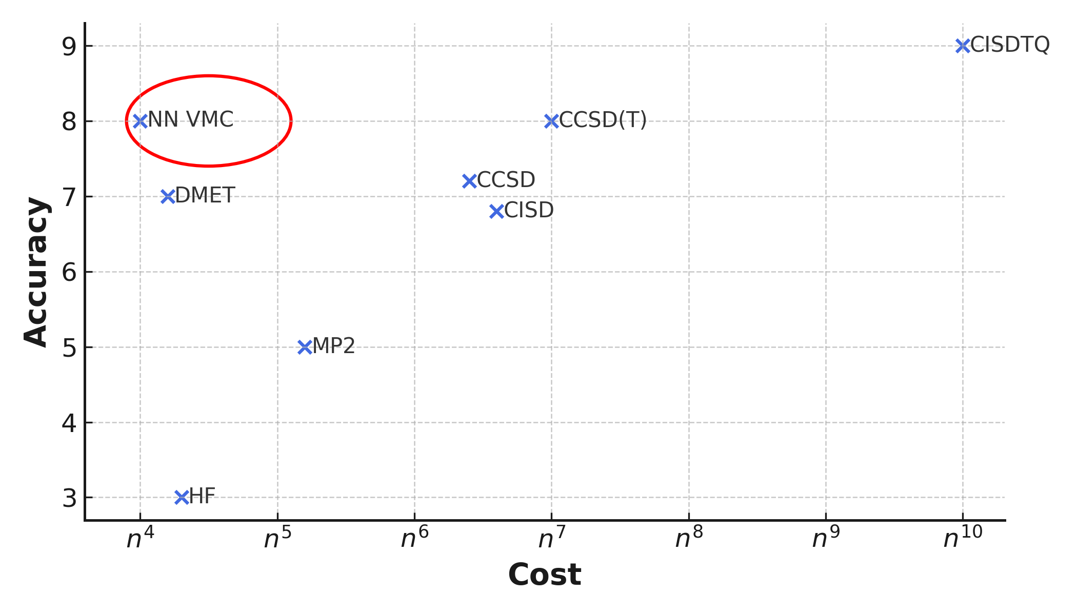Computational cost of different quantum mechanics methods. Note the position of Neural Network Variational Monte Carlo (NN VMC).

To challenge the classical methods, we have developed a machine learning approach to solving the Schrödinger equation. Machine learning is well-suited for this task due to the underlying principles of quantum mechanics:

The variational principle ensures that the system energy \(E\) will never be smaller than the ground-state energy, regardless of the choice of the wavefunction \(\Psi\)

This important because it means we can optimize \(\Psi\) with respect to minimizing \(E\) in order to find the ground state. And once \(E\) is minimized, we have the ground state wavefunction \(\Psi_0\), which in principle provides all the information about the system.

This idea is not innovative. In fact, the foundation of this methodology, known as variational Monte Carlo (VMC), was laid in the 1950’s and has since been very successful (Metropolis & Ulam, 1949). However, the method requires an initial wavefunction guess, or a trial wavefunction, which again requires some insight about the system. Convergence of the method is sensitive to the trial wavefunction, which can be highly non-trivial for complex systems. One way to make the approach more general is to replace the trial wavefunction by a neural network, known for its flexibility (Hornik et al., 1989). The idea was inspired by neural quantum states (Carleo & Troyer, 2017) and FermiNet (Pfau et al., 2020).

For our full paper, please see Front. Phys., 11:1061580.

Machine learning terminology

In machine learning terminology, the trial wavefunction, \(\Psi_T\), is our model. It is represented by a neural network, which contains all the variational parameters that are optimized during training. The associated energy, known as the trial energy, \(E\), will be treated as our loss function and is lower bounded by the ground state energy. I have written a blog post about machine learning, components and terminology.

I asked ChatGPT to generate a brain, where the neurons where replaced by molecules.

Methodology

Machine learning is all about optimizing parameters with respect to minimizing a metric, such as the energy. This is typically done with a gradient method:

\[\theta \leftarrow \theta-\nabla_{E}\Delta x.\]

Here, \(\nabla_{E}\) is the gradient of the energy and \(\Delta_x\) is the step length, or the learning rate in machine learning terms. The energy is computed by solving the inner product

\[E=\frac{\langle\Psi|\hat{\mathcal{H}}|\Psi\rangle}{\langle\Psi|\Psi\rangle},\]

which numerically is possible when we know the wave function \(\Psi\). The algorithm for converging towards the correct ground-state wavefunction \(\Psi_0\) is the following:

1. Initialize the trial wavefunction, \(\Psi_T\), in our case a neural network \(\sim\mathcal{N}(0,\mathbb{I})\)
2. Compute \(E\) from the equation above
3. Compute \(\partial E/\partial\theta\), the gradient components
4. Update \(\Psi\) to minimize the energy
5. Repeat 2, 3 and 4 until convergence

Computation of the energy and the gradients here is the computationally intensive part, and also the mathematically most involved one. This is not needed to follow this blog post, but if you’re curious, feel free to look into the last section.

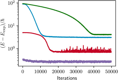
Convergence.

Application: Quantum dots

This method is general, and can in principle be applied to any quantum mechanical system, such as atoms and molecules. However, the system size is limited by the computational cost of the system energy and gradients, and we are in practice restricted to small systems of a few atoms. As a proof of concept, we apply the methodology to quantum dots, which have natural and cheap to calculate basis functions in the Hermite polynomials. Also, the quantum dots have significant applications in the field of technology.

Sampling the energy and gradients*

I will try to keep this post easy to read without too many details, but some math is needed to explain how this method works. However, if you are not familiar with quantum mechanics, feel free to skip this section.

This section is about how the system energy \(E_T\) is calculated for a particular function \(Psi_T\), which is done by sampling.

Suppose that we have an initial guess of our function \(\Psi\), denoted by \(\Psi_T\) (trial function). Then, the trial energy is given by

\[E_T=\int\Psi_T^*\hat{\mathcal{H}}\Psi_T d\tau,\]

where \(E_T\geq E_0\) according to the variational principle, with \(E_0\) as the ground-state energy. By defining the local energy as

\[E_L=\frac{1}{\Psi_T}\hat{\mathcal{H}}\Psi_T,\]

we may write

\[E_T=\int P_T E_L d\tau\]

where the probability distribution follows the Born rule:

\[P_T\equiv \Psi_T^*\Psi_T.\]

An important thing to recognize here is that the trial energy $E_T$ is the expectation value of the local energy $E_L$. This means that the system energy can be found by sampling the local energy:

\[E_T=\langle E_L \rangle = \frac{1}{n}\sum_{i=1}^{n}E_L(i).\]

Here, it is important to draw the system samples from the correct probability distribution \(P_T\), which can be done with Metropolis sampling.

Optimization using machine learning

Once we have calculated the system energy \(E_T\). However, to change \(\Psi_T\) in order to minimize the energy \(E_T\), we need to know how \(E_T\) changes as we change the parameters in \(\Psi_T\), \(\theta\). We need to know \(dE_T(\theta)/d\theta\).

References

1. Carleo, G., & Troyer, M. (2017). Solving the Quantum Many-Body Problem with Artificial Neural Networks. Science (New York, N.Y.), 355(6325), 602. https://doi.org/10.1126/science.aag2302
2. Metropolis, N., & Ulam, S. (1949). The Monte Carlo Method. Journal of the American Statistical Association, 44(247), 335. https://doi.org/10.1080/01621459.1949.10483310
3. Hornik, K., Stinchcombe, M., & White, H. (1989). Multilayer feedforward networks are universal approximators. Neural Networks, 2(5), 359. https://doi.org/10.1016/0893-6080(89)90020-8
4. Pfau, D., Spencer, J. S., Matthews, A. G. D. G., & Foulkes, W. M. C. (2020). Ab initio solution of the many-electron Schr}"odinger equation with deep neural networks. Physical Review Research, 2(3), 033429. https://doi.org/10.1103/PhysRevResearch.2.033429