Computer experiments provide insights that real-world experiments cannot offer. They are also less error-prone and often more cost-effective. This is why computer simulations have become an increasingly popular tool in research. But can we truly rely on these simulations when making important decisions? How can we be sure that computer simulations accurately capture the effects observed in real-world experiments? The answer lies in the fact that simulations must be rigorously tested and validated against real-world data. After all, computer models can never fully replicate all the complexities of the physical world.
Here, we’ll explore computer simulations of water — a substance that is both crucial and notoriously difficult to model. Water is the most abundant liquid on Earth, present in nearly every geological, biological, and environmental context. However, it also exhibits peculiar behaviors that make it a challenge to simulate accurately. These include unusual properties like high surface tension, unusual solvent capabilities, and complex phase transitions — all of which add layers of complexity to modeling efforts.
Water at 300 K, 1 bar pressure.
To address these challenges, most water models are “rigid”, meaning the distance between the oxygen and hydrogen atoms is fixed. This simplifies the model, but it also overlooks critical aspects like chemical reactions, acidity, and other dynamic processes that are essential for realistically simulating water behavior in natural systems. To capture these complexities, we need a more dynamic, dissociative water model. This is precisely what we’ve developed in our recent work, published in the Journal of Physical Chemistry B: here.
The concept of modeling and optimization in science is not new. Charles Darwin famously introduced his theory of evolution 165 years ago, proposing natural selection as the mechanism driving survival of the fittest. While controversial at the time, Darwin’s theory became a cornerstone of modern biology. In addition to the “exploitation” component of natural selection, Darwin acknowledged the importance of “exploration” — driven by mutation and recombination. Inspired by this dual process, we applied a similar approach in optimizing our water model, using a genetic algorithm to evolve and refine it.
Real water molecules can react with the surroundings. Most water models do not capture this chemical nature of water
Reactive water
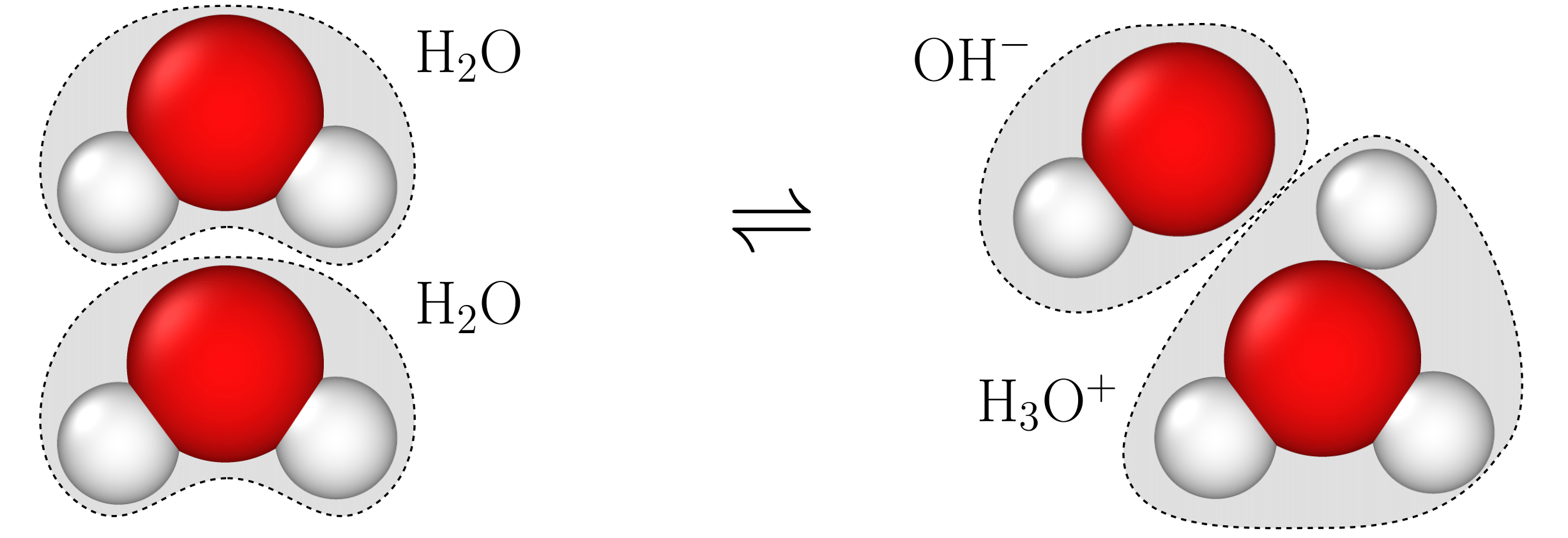
A dissociative water model allows each water molecule to undergo dissociation, meaning water molecules can lose hydrogen atoms to the surroundings, forming hydroxide (OH\(^-\)) groups, or they can accept hydrogen atoms, forming hydronium ions (H\(_3\)O\(^+\)). These reactions can be represented as:
\[\mathrm{H}_2\mathrm{O}\rightleftharpoons\mathrm{OH}^-+\mathrm{H}^+,\]or
\[2\mathrm{H}_2\mathrm{O}\rightleftharpoons\mathrm{H}_3\mathrm{O}^+ + \mathrm{OH}^-.\]These dissociation reactions are fundamental to the behavior of liquid water and are crucial to accurately simulate water in real-world conditions. For example, the acidity of a solution is measured by the pH scale, which defines acidity based on the concentration of hydrogen ions (H\(^+\)). The pH is given by the formula:
\[\mathrm{pH} = -\log\left(\frac{N_{\mathrm{H}^+}}{N}\right),\]where \(N_{\mathrm{H}^+}\) is the number of \(\mathrm{H}^+\) ions and \(N\) is the total number of water molecules. In simpler terms, \(N_{\mathrm{H}^+}/N\) represents the concentration of hydrogen ions. A neutral pH-value is around 7, meaning there is roughly one hydrogen ion per 10 million water molecules. In contrast, an acidic solution with a pH of 4 will have one hydrogen ion per 10,000 water molecules, and the concentration increases as the pH decreases.
An all-atom water model
How can we accurately capture the behavior of water in a model? One approach might be to allow an atom to detach from a molecule if the force on it exceeds a certain threshold. However, this method would result in a binary attachment-detachment dynamic, which ultimately does not reflect the true physical behavior of water. A more realistic solution is to use an all-atom model, where every atom is treated independently, and the concept of a fixed molecule is not necessary. In this model, atoms follow the same physical laws whether they are part of a molecule or free. This approach better aligns with how atoms behave in nature.
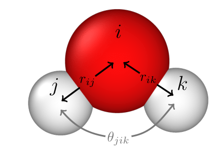 The force acting on a particle \(i\) is determined by the distance to its neighbor atoms, \(r_{ij}\) and \(r_{ik}\), and the angle between three atoms \(\theta_{jik}\)
We have used the Vashishta model to describe the interactions between atoms, which accounts for four distinct forces acting between any two atoms:
- Charge-charge force (Coulomb), \(\propto 1/r^2\)
- Change-dipole force, \(\propto 1/r^5\)
- Dipole-dipole force (van der Waals force), \(\propto 1/r^7\)
- Repulsive force steming from the overlap of electron clouds, \(\propto ~1/r^{12}\)
Here, \(r\) represents the distance between two atoms. It’s important to note that all these forces are Coulombic in nature. However, since each atom is treated as a charged point particle, electron polarization is not accounted for.
The total potential energy between two atoms is described by:
\[V_{ij}^{(2)}(r)=\frac{H_{ij}}{r^{\eta_{ij}}}+\frac{Z_iZ_j}{r}e^{-r/\lambda_1}-\frac{D_{ij}}{2r^4}e^{r/\lambda_4}-\frac{W_{ij}}{r^6},\]where \(H_{ij}\), \(\eta_{ij}\), \(Z_i\), \(Z_j\), \(\lambda_1\), \(D_{ij}\), \(\lambda_4\) and \(W_{ij}\) are parameters specific to the water model. While the exact functional form of the interaction is not the focus here, the key takeaway is that for each combination of atom types, there are 8 parameters that need to be determined.
In addition to these pairwise interactions, a force is introduced when more than two atoms are present. This is especially important for modeling angles between atoms, which is crucial for simulating the structure of water. The interaction is modeled with an angular spring term, which maintains an equilibrium angle:
\[V_{jik}^{(3)}(r_{ij}, r_{ik}, \theta_{jik})=B_{jik}\exp\left(\frac{\gamma}{r_{ij}-r_0}+\frac{\gamma}{r_{ik}-r_0}\right)\frac{(\cos\theta_{jik}-\cos\bar{\theta}_{jik})^2}{1+C_{jik}(\cos\theta_{jik}-\cos\bar{\theta}_{jik})^2},\]where \(B_{jik}\), \(\gamma\), \(r_0\), \(\cos\bar{\theta}_{jik}\) and \(C_{jik}\) are parameters that must be determined. Additionally, a cutoff distance parameter, \(r_c\), is introduced to disregard interactions between atoms that are farther apart than this threshold.
In total, for each possible three-atom combination, there are 14 parameters to be determined. For water, with two atom types (hydrogen and oxygen), there are \(2^3=3\) possible three-atom combinations, resulting in 112 parameters in total. Some of these parameters are equivalent due to symmetries, and others can be inferred from experimental data. However, there are still many parameters to optimize, far more than can be tackled with a simple grid search. To address this complexity, we need a more systematic approach.
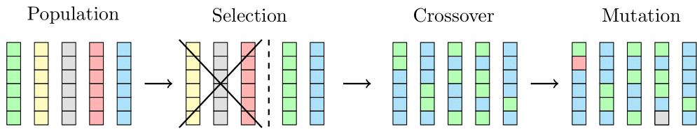
One generation of the genetic algorithm: We begin with an initial population of 5 individuals. First, the fittest individuals are identified using an objective fitness score, and those that don’t meet the standard are discarded. Next, crossover occurs between their chromosomes (represented by colored boxes here), which simulates the exploitation aspect of evolution. Finally, random mutations are applied to the chromosomes, representing the exploration aspect before the next generation is formed
Global optimization using a genetic algorithm
Inspired by the principles of evolution, we use a genetic algorithm to find the optimal values for the parameters. Charles Darwin’s theory of evolution posits that biological evolution is driven by natural selection, where only the fittest individuals survive and reproduce, reinforcing advantageous traits in each generation. When two individuals mate, their genomes are mixed in a seemingly random fashion, exploiting the existing knowledge encoded in their genes. Additionally, the exploration aspect of evolution is represented by random mutations, where some genes are altered independently of the parent genomes.
In the context of our model, genetic algorithms work in a similar way. Each individual represents a set of parameters, and starting with a population of \(N\) individuals, the fitness of each individual is calculated using an objective score. Only the fittest individuals reproduce, ensuring that each new generation is built from the strongest members of the previous one. Additionally, random mutations are introduced to some parameters to help the algorithm explore the solution space more effectively.
Objective fitness score
A key component of the genetic algorithm is the objective fitness function, which determines how “good” an individual is in relation to the problem at hand. In our case, each individual is a parameterization of the Vashishta potential, and the fitness score reflects how closely each parameterization matches the experimental values for bulk water density across different temperatures and pressures. The process of calculating the density requires molecular dynamics simulations, which is the most computationally expensive part of the genetic algorithm.
Since we are optimizing multiple quantities simultaneously, the objective fitness function is composed of several terms. A straightforward approach would be to weight all terms equally and calculate them all at once. However, we can save considerable computational resources by prioritizing certain quantities and gradually adding those of lower priority once the higher-priority ones are optimized. This approach is a fundamental feature of the Hierarchical Objective Genetic Algorithm (HOGA).
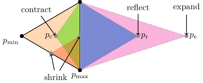 The Nelder-Mead simplex algorithm is based on evaluating three points close to each other in the parameter space. Here, \(p_{\mathrm{min}}\) is the point with the lowest fitness value and \(p_{\mathrm{max}}\) is the point with the highest fitness value. The algorithm involves four possible actions, all of which include adjusting \(p_{\mathrm{min}}\): moving \(p_{\mathrm{min}}\) by contraction (green), reflection (blue), or expansion (pink), or shrinking the simplex towards \(p_{\mathrm{max}}\) (red)
Local optimization
Once the fitness score has reached an acceptable value, we have located a satisfactory local minimum in the parameter space. To refine this minimum further, we employ a local optimization technique based on the Nelder-Mead simplex method. The concept is straightforward: we begin by evaluating three points near the best solution we’ve found so far, which is why it’s called a “simplex”. Based on the results, we move one of the points (vertices) and form a new simplex using one of the following four actions:
- Reflect
- Contract
- Expand
- Shrink
The action to be taken is determined by a set of rules designed to exploit the current knowledge while also encouraging exploration. By iterating through these steps, the new simplex should ideally have a better fitness score than the previous one. This process continues until the algorithm converges to a solution.
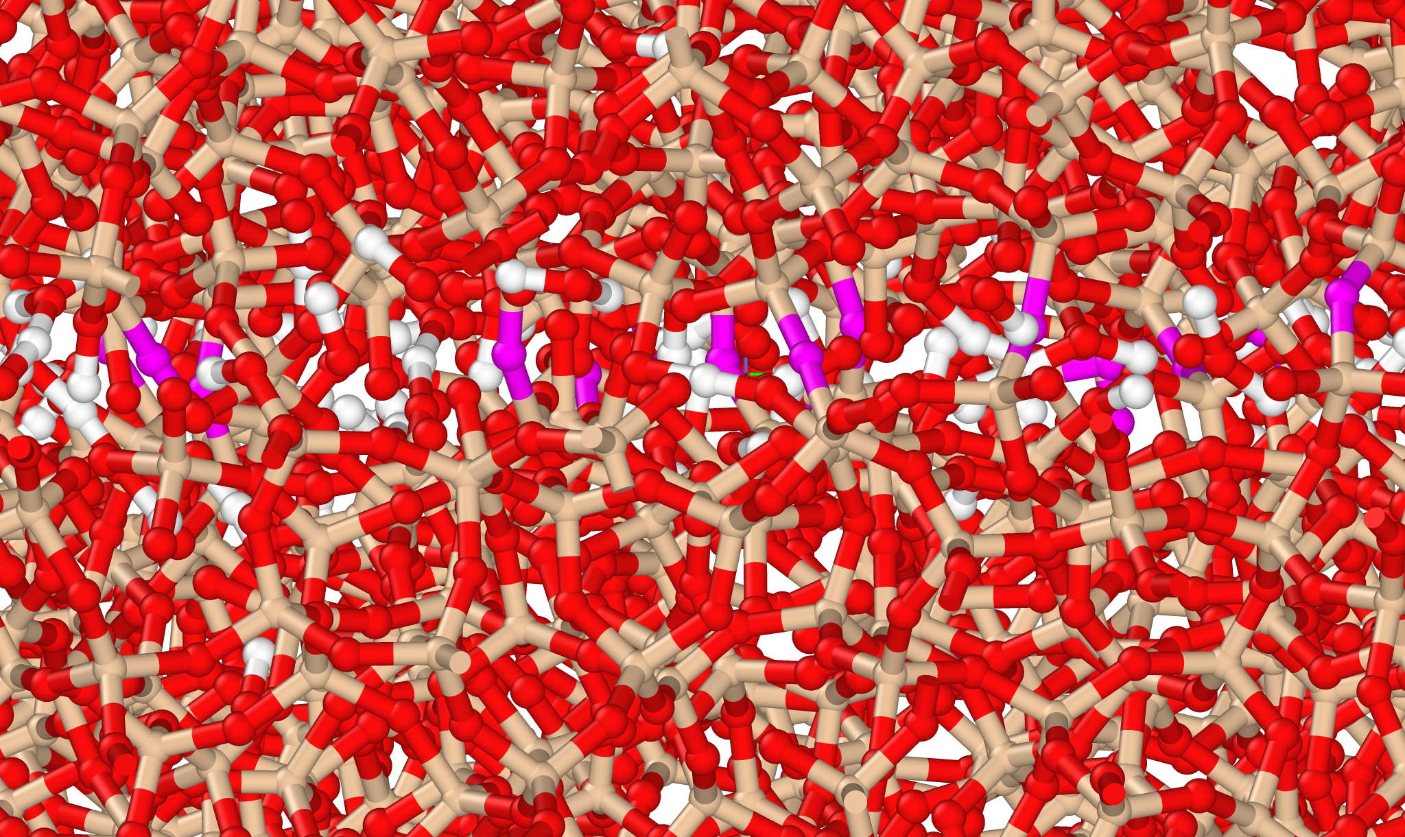
With a reactive water potential, we can simulate interactions with other components. Here, water is simulated alongside silicon dioxide, forming siloxane bonds (purple). These siloxane bonds play a significant role in frictional aging, as discussed on my friction page.
Adding more components
What if we want to simulate more than just water? The process can be extended to include additional components. However, each time we add a new component, we must determine the interaction parameters between the new component and the existing components, as well as within the new component itself. For example, adding a third component introduces new three-atom combinations, increasing the number of parameters that need to be optimized.
As we add more parameters to optimize, the complexity of the optimization task increases exponentially. In general, this makes it difficult to expand the model with additional components. However, by leveraging physical intuition, we can often reduce the dimensionality of the problem, making the task more manageable.
For example, we know that water molecules must be charge-neutral, meaning that the charges on hydrogen (\(Z_{\mathrm{H}}\)) and oxygen (\(Z_{\mathrm{O}}\)) atoms must be related by the equation:
\[2Z_{\mathrm{H}}=-Z_{\mathrm{O}}.\]When modeling geological systems, the interaction between water and silicon dioxide (silica) is particularly important. To simulate this, we can add silicon as a new component to the water model, following the same optimization procedure described above.
Vaporization properties
Measuring vaporization properties of the water potential using molecular dynamics simulations is challenging, as nucleation events are inheritly rare. Instead, those kind of events can be quantified using biased Monte Carlo sampling. More information on that cna be found in: Camposano, Nordhagen, Sveinsson, Malthe-Sørenssen, An Extended Energy-Biased Aggregation-Volume-Bias Monte Carlo (EB-AVBMC) Method for Nucleation Simulation of a Reactive Water Potential, J. Chem. Theory Comput. (2025), 21, 14, 6769–6776
Conclusions
Computer simulations provide valuable insights and information that are often inaccessible through real experiments. However, to achieve reliable results, the model used to describe atomic interactions must be carefully calibrated. In this project, we explored how a reactive water model can be developed using a method inspired by Darwin’s theory of evolution. Additionally, this model can be extended to include more components.
For more details, please read our paper published in Journal of Physical Chemistry B: Camposano, Nordhagen, Sveinsson, Malthe-Sørenssen, Genetic Algorithm Workflow for Parameterization of a Water Model Using the Vashishta Force Field, J. Phys. Chem. B (2025), 129, 4, 1331–1342.
Disclaimer: All illustrations used here were created with Ovito and TikZ.
Feel free to drop a comment or question below if you have thoughts or experiences you’d like to share.
