Bris

Can recent breakthroughs in data-driven weather forecasting be replicated at high spatial resolution?

Over the last few years, data-driven weather models have shown impressive forecast skill at a fraction of the computational cost of traditional numerical weather prediction (NWP) systems. Most of these models, however, are trained on ERA5 reanalysis data with a relatively coarse horizontal resolution of about 31 km. This raises a natural and important question: can similar performance be achieved at much higher resolution, where fine-scale weather phenomena are explicitly resolved?

In this post, I introduce Bris, a high-resolution probabilistic data-driven weather model trained on the MetCoOp Ensemble Prediction System (MEPS) analysis at 2.5 km resolution. The name Bris means breeze in Norwegian and is pronounced accordingly—it is not an acronym. The work is a collaboration between the Norwegian Meteorological Institute (MET Norway) and the European Centre for Medium-Range Weather Forecasts (ECMWF).

To generate physically realistic weather scenarios, we designed a training objective that combines probabilistic accuracy with spatial and spectral consistency. The resulting model matches the forecast skill of MEPS while running roughly 20–30× faster. Below, I outline the motivation, model design, and key results, and discuss where this approach is headed next.

I aim to explain the ideas in accessible language. For a more technical treatment, see our recent preprint (Nordhagen et al., 2025). The methodology also builds on the stretched-grid approach discussed in an earlier post.

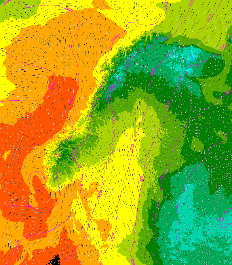
Example forecast field produced by Bris. Color palete indicates 2m temperature, contour lines are mean sea level pressure and streamlines indicate 10m wind.

The case for high resolution

Why invest in high-resolution models when state-of-the-art global models already perform so well?

The answer depends on both the variable and the application. Some atmospheric quantities, such as precipitation, near-surface wind, and local temperature extremes, vary strongly over short distances. Accurately representing this variability requires high spatial resolution. This is why many national meteorological and hydrological services operate convection-permitting regional models.

Other variables, such as mean sea level pressure, are dominated by large-scale atmospheric structures. For these, increasing resolution yields limited benefit. To illustrate this contrast, we compare Bris (2.5 km resolution) with ECMWF’s data-driven model AIFS-CRPS at 31 km resolution (Lang et al., 2024):

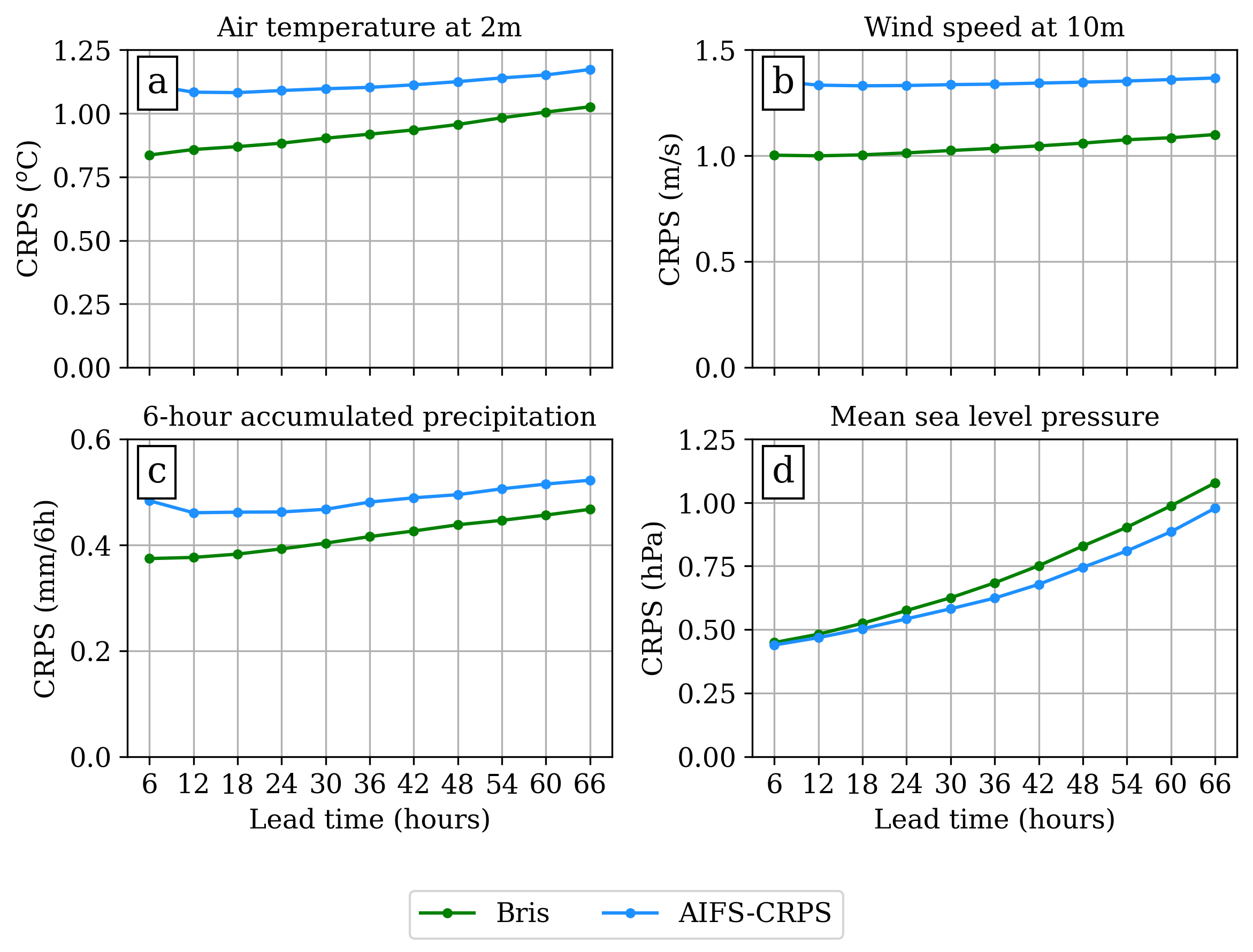
Continuous Ranked Probability Score (CRPS) for 2 m temperature, 10 m wind speed, 6-hour accumulated precipitation, and mean sea level pressure, verified against synoptic stations in Norway. Lower scores indicate better performance.

CRPS is a proper scoring rule for probabilistic forecasts; it measures both accuracy and uncertainty. Bris shows clear improvements for temperature, wind speed, and precipitation, while performing slightly worse for mean sea level pressure. Since AIFS-CRPS is a state-of-the-art global model, this comparison highlights where high resolution adds real value.

High resolution is especially important for extreme weather events, such as heavy precipitation and strong winds, which cause significant societal impacts each year. Given that protecting life and property is a core responsibility of national meteorological services, high-resolution probabilistic forecasting remains essential.

Why probabilistic forecasting?

Weather models can be either deterministic, producing a single forecast, or probabilistic, estimating the likelihood of multiple possible outcomes.

The atmosphere is a chaotic system influenced by inherently unpredictable processes such as turbulence. In the language of chaos theory, it is often described as a level-1 chaotic system: its future evolution is sensitive to random processes beyond our control. Even if the governing equations were perfectly deterministic, measurement errors and incomplete knowledge of the initial state would still limit predictability.

Edward Lorenz famously illustrated this sensitivity using a simple nonlinear system, showing that tiny perturbations can lead to vastly different trajectories - the so-called butterfly effect:

Two nearly identical initial states diverge rapidly, illustrating sensitivity to initial conditions.

Because of this intrinsic uncertainty, forecasting probabilities rather than single outcomes provides a more faithful description of future weather. Probabilistic forecasts offer three key advantages:

1. Explicit quantification of uncertainty
2. Sharper, more physically consistent forecast fields
3. Improved representation of rare and extreme events

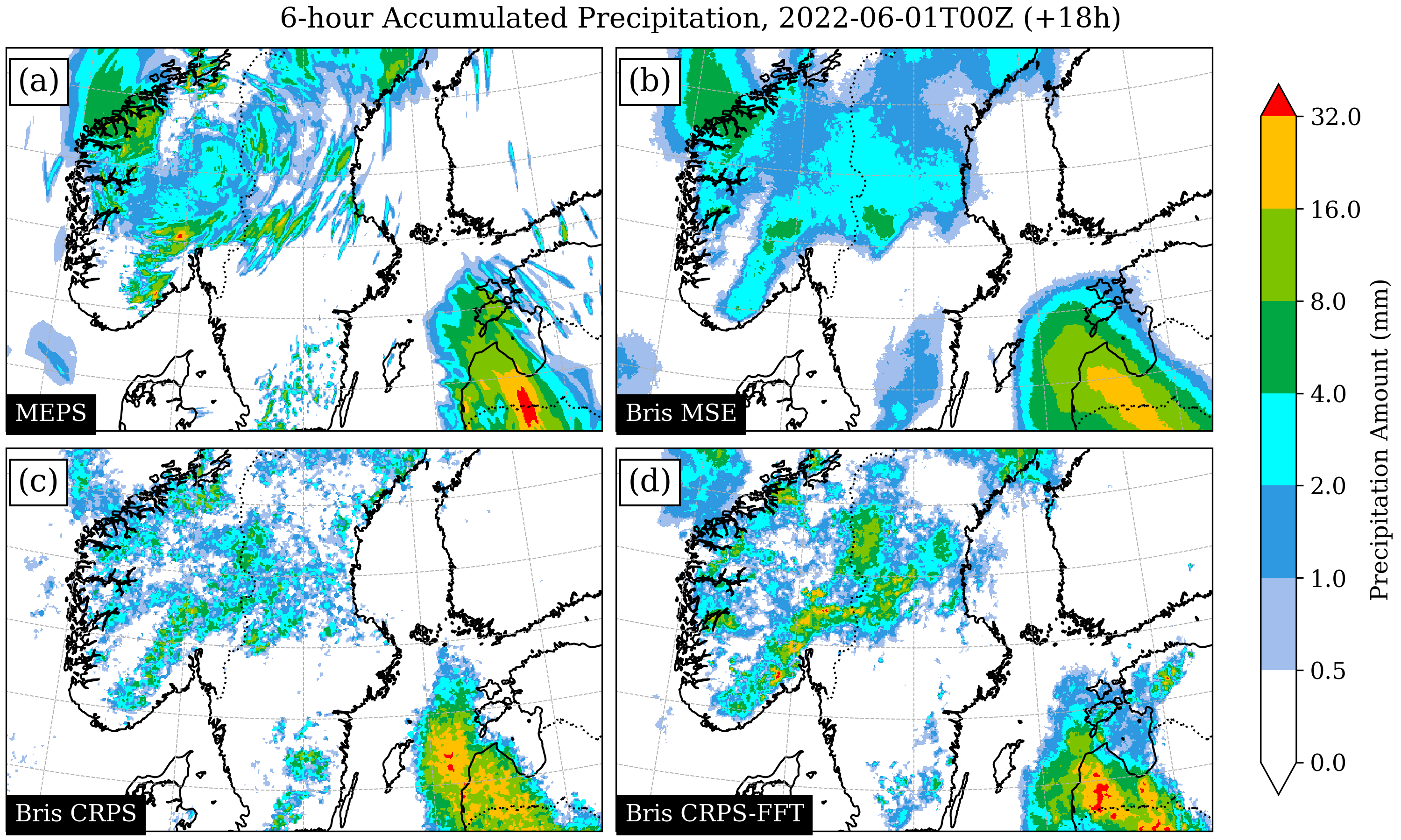
Precipitation forecasts at 2.5 km resolution. Panels show (a) MEPS, (b) a deterministic model, (c) Bris trained with a simplified loss, and (d) Bris trained with the full probabilistic objective.

Probabilistic forecasts are commonly implemented as ensemble prediction systems (EPS), where each ensemble member represents a plausible future trajectory. Probabilities are derived by analyzing the distribution of these members.

Deterministic models are typically trained using mean squared error, which encourages predictions close to the ensemble mean. While effective in many settings, this often produces overly smooth fields that do not correspond to any physically realistic atmospheric state, a phenomenon known as the double penalty effect.

How Bris works

Bris follows an encoder–processor–decoder architecture, with each component implemented as a graph neural network (GNN):

Bris is based on an encoder-processor-decoder design, like other leading data-driven models for weather prediction.

Model architecture

The model takes atmospheric states at −6 h and 0 h as input, with shape \((2, N_\text{grid}, N_\text{var}),\) where \(N_\text{grid} \approx 1.4 \times 10^6\) and \(N_\text{var} = 103\). The encoder maps these fields to a latent representation of shape \((N_\text{mesh}, N_\text{channels}),\) with \(N_\text{mesh} \approx 2.8 \times 10^5\) and \(N_\text{channels} = 1024.\)

This design reduces spatial dimensionality while increasing representational depth. The latent space is intentionally rich: rather than heavily compressing the input, we allow the model to represent complex nonlinear dynamics as approximately linear interactions in a high-dimensional space. Empirically, this significantly improves forecast skill.

Graph neural network formulation

The model operates on a graph where nodes represent spatial locations and edges represent interactions:

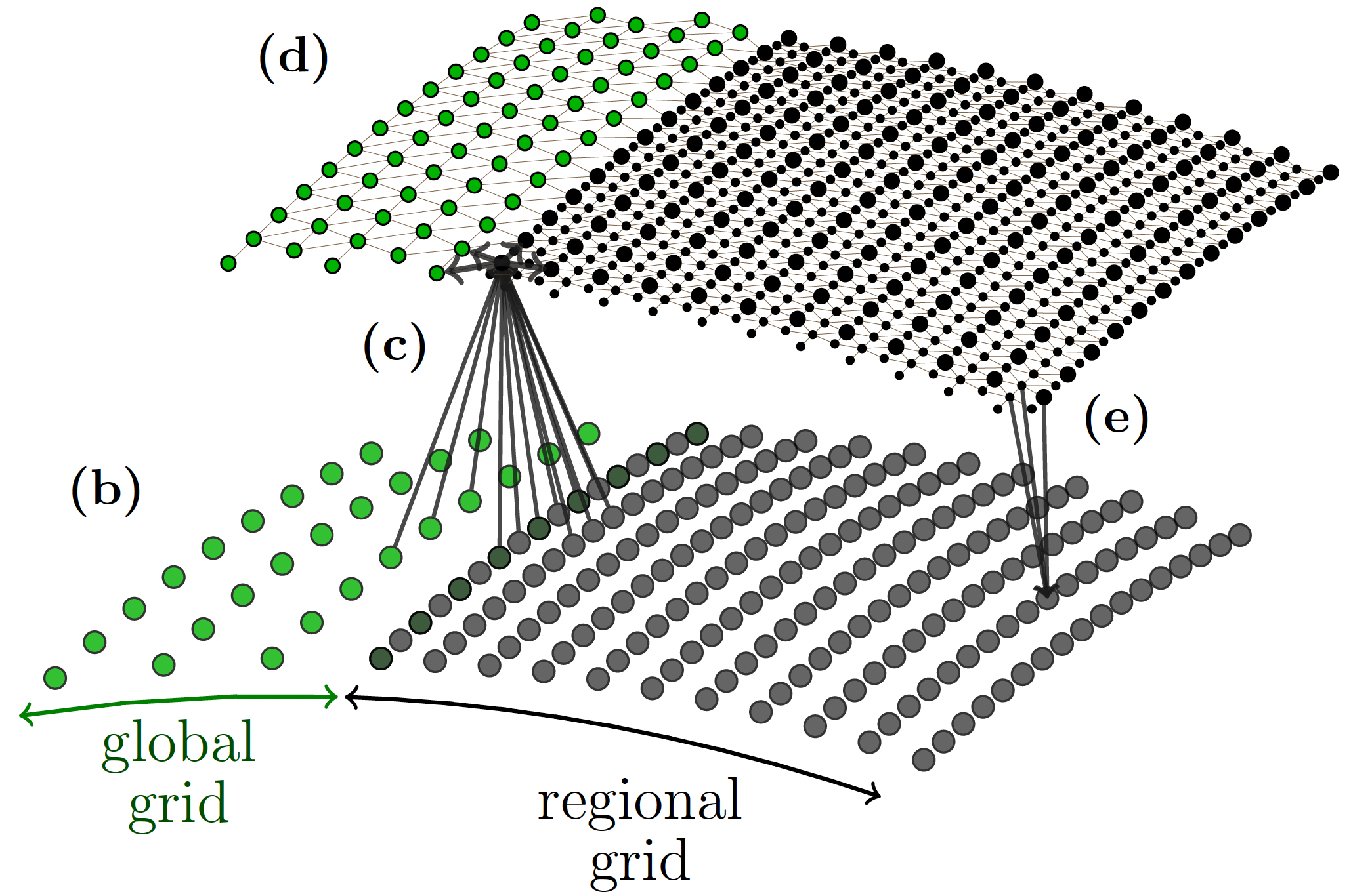
Grid nodes are connected to latent nodes by encoder edges; latent nodes interact via processor edges; decoder edges map back to grid space.

All trainable parameters reside in the edge functions. Encoder edges, processor edges, and decoder edges each share parameters across space, making the model largely position-agnostic. This has two major benefits:

1. Strong generalization across regions, terrains, and climates
2. Flexibility to change the underlying graph between training and inference

In practice, this allows us to pretrain on a global domain and fine-tune on a high-resolution regional grid, or to deploy the model in new regions with minimal modification.

Schematic of the encoder-processor-decoder design and ensemble training. (a) Inputs are past (\(t_{−6h}\)) and current (\(t_{0h}\)) states from MEPS and ERA5, replicated M times for ensemble members. (b) The encoder-processor-decoder architecture injects noise (z) into the latent space to model stochasticity. (c) Predictions are evaluated using point-wise and spectral loss functions.

Ensemble generation and training objective

To generate an ensemble, we inject stochastic noise into the latent space. Physically, this represents unresolved and stochastic atmospheric processes.

A well-calibrated ensemble has small spread when predictability is high and larger spread when uncertainty increases. During training, we explicitly optimize for this behavior using the Continuous Ranked Probability Score (CRPS), a proper scoring rule defined as

\[\mathrm{CRPS}(F, y) = \int_{-\infty}^{\infty} \left( F(z) - \mathbf{1}\{z \ge y\} \right)^2 \, \mathrm{d}z.\]

For an ensemble \(\{x_1, \ldots, x_M\}\), CRPS can be decomposed into accuracy and spread terms (Gneiting & Raftery, 2007):

\[\mathrm{CRPS} = \frac{1}{M} \sum_{m=1}^{M} |x_m - y| - \frac{1}{2M^2} \sum_{m=1}^{M} \sum_{n=1}^{M} |x_m - x_n|.\]

Optimizing CRPS point-wise ensures good marginal distributions, but alone it can lead to noisy spatial fields. To address this, we also evaluate CRPS in spectral space using the fast Fourier transform (FFT). The final loss combines point-wise and spectral terms over global and regional domains:

\[\mathcal{L} = \sum_v \sum_t w_v \Big[ \mathrm{CRPS}_\text{global} + \lambda_r \big( \mathrm{CRPS}_\text{regional} + \lambda_f \, \mathrm{CRPS}_\text{spectral} \big) \Big].\]

This combination preserves probabilistic calibration while enforcing spatial coherence.

Comparison with NWP

We evaluate Bris against the operational MEPS ensemble, focusing on variables most relevant for public forecasting: temperature, wind speed, precipitation, and mean sea level pressure.

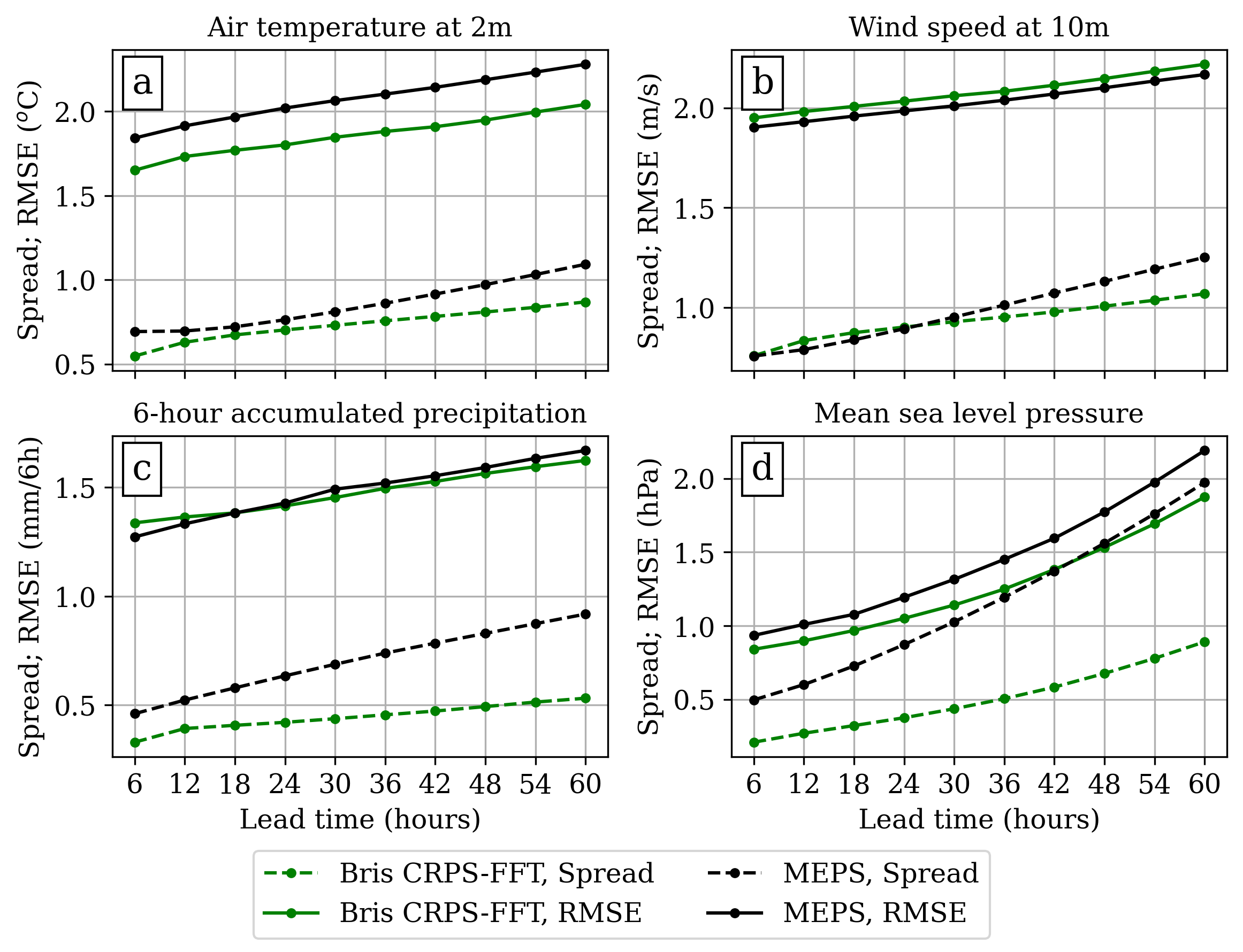
Ensemble spread and RMSE of the ensemble mean for Bris and MEPS. In a perfectly calibrated system, the curves overlap.

Bris achieves lower RMSE than MEPS for most variables, with particularly strong improvements for temperature at lead times up to 36 hours. Wind speed performance is comparable, with a slight degradation in some ranges. Both systems exhibit underdispersion, though Bris has systematically smaller spread—an issue we are actively addressing.

Operational status

Bris has been running operationally four times per day at MET Norway since October 2025 for internal evaluation. It produces the same core outputs as the operational NWP system:

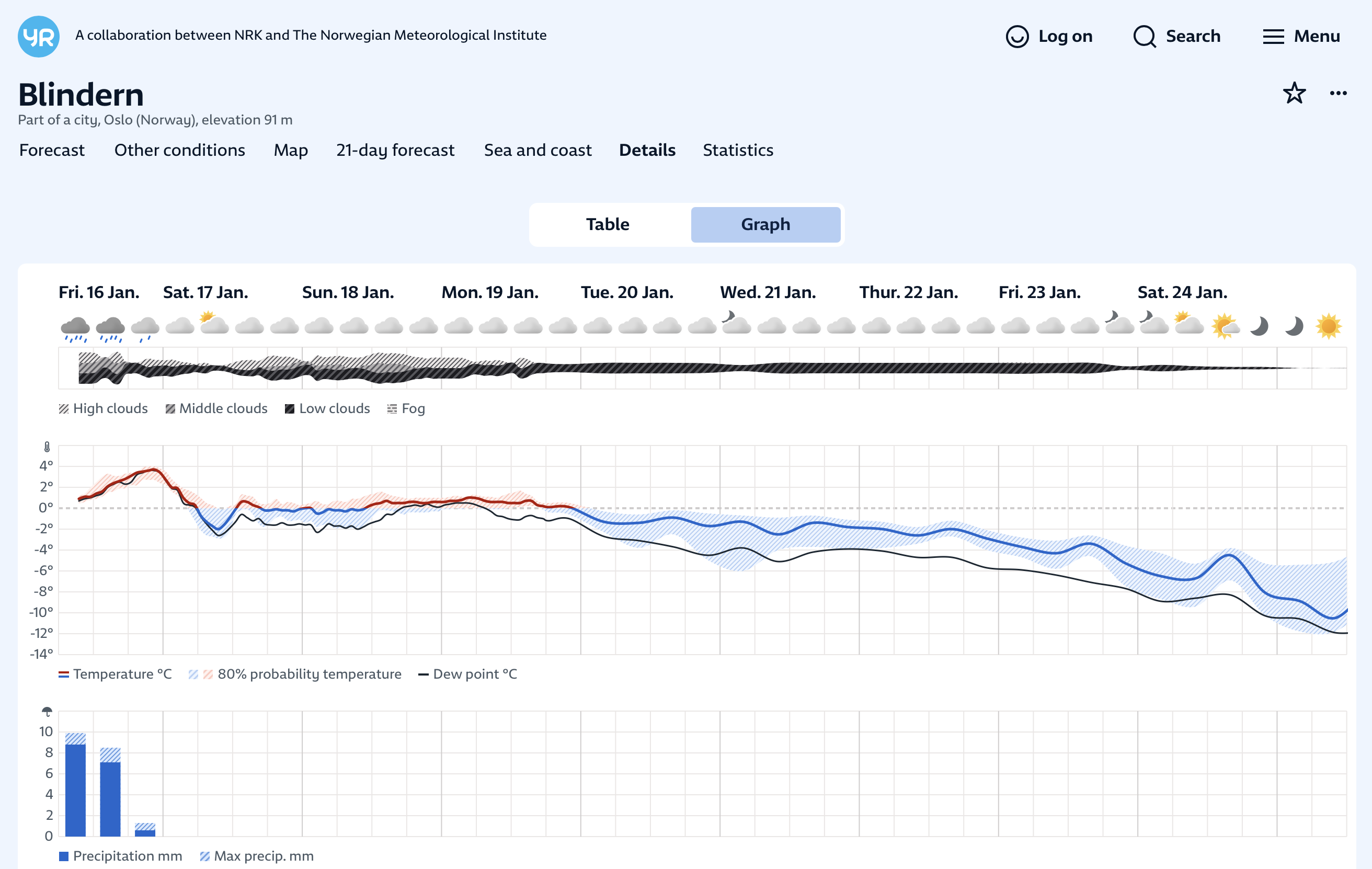
Example temperature and precipitation forecasts with uncertainty.

Although Bris operates at 6-hour temporal resolution, we use a learned time interpolator to produce hourly forecasts. This interpolator is trained on hourly data and will be discussed in a future post.

Conclusions

Bris demonstrates that high-resolution probabilistic data-driven models can be competitive with state-of-the-art NWP systems while being orders of magnitude faster. By combining graph-based architectures with a physically informed probabilistic training objective, we obtain sharp, coherent, and well-calibrated forecasts at convection-permitting scales.

---

DOI: https://doi.org/10.5281/zenodo.18297260
Archived version: Zenodo
Canonical version: https://evennordhagen.com/2026-01-19-bris/

Feel free to leave a comment or question below.

References

1. Lam, R., Sanchez-Gonzalez, A., Willson, M., Wirnsberger, P., Fortunato, M., Alet, F., Ravuri, S., Ewalds, T., Eaton-Rosen, Z., Hu, W., Merose, A., Hoyer, S., Holland, G., Vinyals, O., Stott, J., Pritzel, A., Mohamed, S., & Battaglia, P. (2023). Learning skillful medium-range global weather forecasting. Science, 382(6677), 1416–1421. https://doi.org/10.1126/science.adi2336
2. Bi, K., Xie, L., Zhang, H., Chen, X., Gu, X., & Tian, Q. (2023). Accurate medium-range global weather forecasting with 3D neural networks. Nature, 619(7970), 533–538. https://doi.org/10.1038/s41586-023-06185-3
3. Nordhagen, E. M., Haugen, H. H., Salihi, A. F. S., Ingstad, M. S., Nipen, T. N., Seierstad, I. A., Frogner, I.-L., Clare, M., Lang, S., Chantry, M., Dueben, P., & Kristiansen, J. (2025). High-Resolution Probabilistic Data-Driven Weather Modeling with a Stretched-Grid. arXiv. https://doi.org/10.48550/arXiv.2511.23043
4. Lorenz, E. N. (1963). Deterministic Nonperiodic Flow. Journal of the Atmospheric Sciences, 20, 130–148. https://doi.org/10.1175/1520-0469(1963)020<0130:DNF>2.0.CO;2
5. Lang, S., Alexe, M., Clare, M. C. A., Roberts, C., Adewoyin, R., Bouallègue, Z. B., Chantry, M., Dramsch, J., Dueben, P. D., Hahner, S., Maciel, P., Prieto-Nemesio, A., O’Brien, C., Pinault, F., Polster, J., Raoult, B., Tietsche, S., & Leutbecher, M. (2024). AIFS-CRPS: Ensemble forecasting using a model trained with a loss function based on the Continuous Ranked Probability Score. arXiv. https://doi.org/10.48550/arXiv.2412.15832
6. Bonev, B., Kurth, T., Mahesh, A., Bisson, M., Kossaifi, J., Kashinath, K., Anandkumar, A., Collins, W. D., Pritchard, M. S., & Keller, A. (2025). FourCastNet 3: A geometric approach to probabilistic machine-learning weather forecasting at scale. arXiv. https://doi.org/10.48550/arXiv.2507.12144
7. Gneiting, T., & Raftery, A. E. (2007). Strictly Proper Scoring Rules, Prediction, and Estimation. Journal of the American Statistical Association, 102(477), 359–378. https://doi.org/10.1198/016214506000001437