Artificial intelligence (AI) has enabled us to tackle problems that seemed impossible just a decade ago. It has revolutionized fields such as natural language processing, image synthesis, video generation, and weather forecasting — the area I’m currently most involved in. In this blog post, we’ll explore what AI really is, its key components, the current state of the field, future directions, and the role Python plays in AI development. I’ll also include a tribute to my brilliant informatics lecturer, Hans Petter Langtangen.
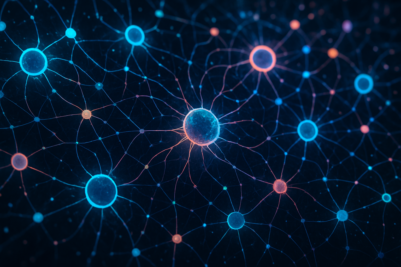
Artificial intelligence, particularly neural networks, is inspired by the structure and function of the human brain’s neural networks, but only loosely emulates them
I began my physics studies at the University of Oslo (UiO) in 2014, where we were fortunate to be introduced to programming from the very first semester. From the outset, we were essentially trained to become computational physicists. At that time, a significant debate was unfolding within the Faculty of Mathematics and Natural Sciences regarding which programming language should be taught to bachelor students. Many professors advocated for low-level languages like C, C++, and Fortran, citing their speed and prevalent use in physics applications.
To be fair, these languages were the natural choice back then, holding a much higher market share than higher-level, slower alternatives like Python and MATLAB. However, Hans Petter Langtangen presented a compelling argument for Python. He emphasized that Python encompasses all the necessary components suitable for students without prior programming experience. As a scripting language, it is pre-compiled, facilitates easy integration of third-party code, and is open-source. Despite Python’s modest market share of only 2% at the time, Langtangen successfully persuaded his colleagues to adopt it for teaching. As we will soon see, that decision proved to be a very wise one.
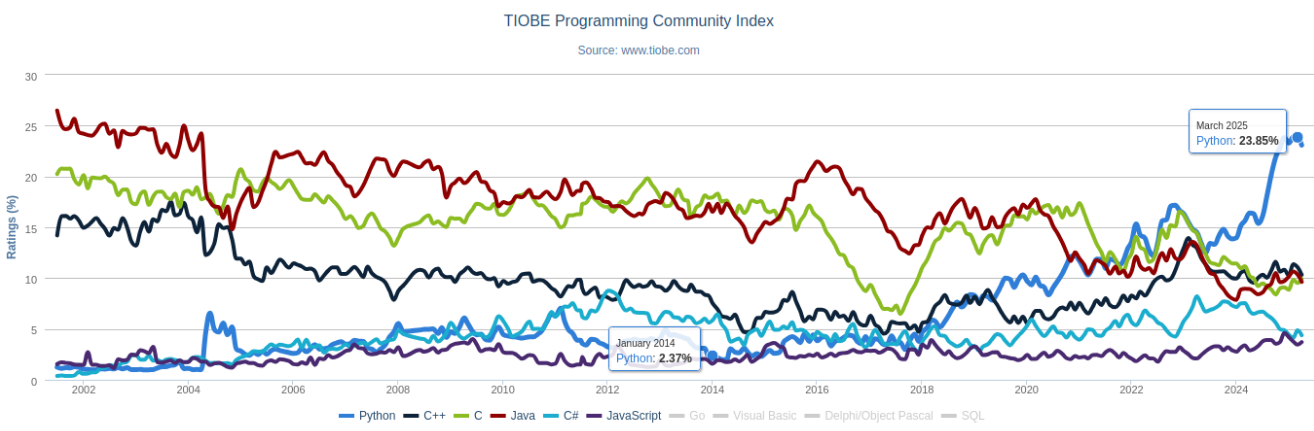
Python’s TIOBE rating has increased from 2.4% in 2014 to 23.8% in 2025. Source: tiobe.com
The popularity of Python has skyrocketed in recent years, largely driven by the rise of artificial intelligence—especially machine learning. Today, the vast majority of large-scale machine learning projects (over 90%) are developed in Python. In a sense, machine learning is synonymous with Python—whether you like it or not.
But the relationship goes both ways. Python has been just as crucial to the growth of machine learning as machine learning has been to Python’s success. Much of the field’s rapid progress is thanks to powerful open-source libraries developed by the Python community—such as PyTorch, TensorFlow, and JAX—all of which embody Python’s core philosophy of simplicity and readability. Combined with advances in hardware, these libraries are a key reason why machine learning development is evolving at such a fast pace.
Exactly what is machine learning?
So, what exactly is machine learning? In simple terms, machine learning is the science of training computers to perform tasks without being explicitly programmed. Typically, this involves optimizing a complex function based on a specific metric using an algorithmic approach.
Sound confusing? Don’t worry—there’s a concrete example coming up that should make things clearer.
Although the term machine learning feels modern, many of its underlying techniques have been around for decades. For example, basic gradient descent—a core optimization method—has been used since the early days of calculus and falls squarely under the machine learning umbrella.
What’s truly new is our ability to train deep artificial neural networks, a subfield known as deep learning. Much of the recent progress in AI stems from this advancement—but we’ll save a deeper dive into deep learning for later.
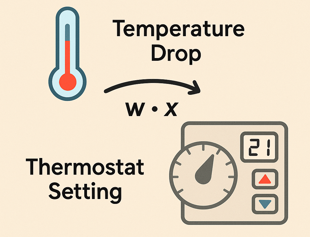
In the example below, machine learning is used to find the optimal thermostat setting, given the temperature change outside.
Example: Tuning a Thermostat
Let’s look at a simple example to illustrate how machine learning works. Since I work in weather prediction, we’ll use a temperature-related scenario:
Imagine you have a thermostat inside your house that needs to be adjusted based on the outside temperature. When the outside temperature drops, you need to increase the thermostat setting to maintain a constant indoor temperature. Conversely, when the outside temperature rises, you should lower the thermostat. But exactly how much should you adjust it?
To answer that, you collect some data. You find that when the outside temperature drops by 2°C, the thermostat must be increased by 3°C to maintain comfort. You observe similar patterns for other temperature changes:
| \(i\) | Outside Temp Drop (°C) | Thermostat Increase (°C) |
|---|---|---|
| 1 | 2 | 3 |
| 2 | 5 | 7 |
| 3 | 7 | 10 |
| 4 | 10 | 13 |
| 5 | 1 | 1.5 |
Although this is a classic linear regression problem with an analytical solution, let’s solve it using a machine learning approach. We want a model that predicts the thermostat increase as a function of the temperature drop:
\(\hat{y}_i=w\cdot x_i\),
Here, \(x_i\) is the outside temperature drop, \(\hat{y}_i\) is the predicted thermostat increase, and \(w\) is the parameter we want to learn. We’ll optimize \(w\) by minimizing a loss function, in this case the mean squared error:
\(\mathcal{L}(w)=\frac{1}{5}\sum_{i=1}^5(y_i-wx_i)^2\).
Let’s start with an initial guess of \(w=1\). The loss becomes:
\(\mathcal{L}(1)=\frac{1}{5}((3-2)^2+(7-5)^2+(10-7)^2+(13-10)^2+(1.5-1)^2)=4.65\).
This value tells us that the squared error is 4.65°C\(^2\) on average. Now we compute the gradient of the loss with respect to \(w\):
\[\nabla_w\mathcal{L}(w) = -\frac{2}{5}\sum_{i=1}^5(y_i-wx_i)\cdot x_i\]Plugging in \(w=1\):
\(\nabla_w\mathcal{L}(1) = -\frac{2}{5}(2+10+21+30+0.5)=-25.4\).
The negative gradient means that increasing \(w\) will reduce the loss. We can now update \(w\) using gradient descent:
\(w\leftarrow w-\eta\nabla_w\mathcal{L}(w)\),
where \(\eta\) is the so-called learning rate. This iterative process continues until the loss converges to a minimum. By adjusting \(w\) iteratively, we will see that the optimal value in this problem is \(w=1.35\). So for every degree the outside temperature drops, we need to increase the thermostat by 1.35°C.
This is an example of an extremely basic machine learning problem, but it illustrates the concepts, including the data, model, loss function and learning rate. In practice, typical machine learning problems include large amounts of data and a much more complex model, often based on neural networks.
An artificial neural network
It’s difficult to discuss recent advances in machine learning without mentioning artificial neural networks. Inspired by the structure of the brain, these networks consist of interconnected nodes (or “neurons”) that transmit signals and activate in response to specific inputs.
More importantly, neural networks—henceforth referred to simply as neural networks—are universal function approximators. This means they are flexible enough to approximate any continuous function, as shown by Hornik et al. (Hornik et al., 1989).
A simple example is the two-layer perceptron, which can be expressed mathematically as:
\(\hat{y}_i=a^{(2)}\left(\sum_jw_{ij}^{(2)}\left(a^{(1)}\left(\sum_k w_{jk}^{(1)} \cdot x_k\right)\right)\right)\).
Here:
- \(w^{(1)}\) and \(w^{(2)}\) are the weight matrices for the first and second layers, respectively.
- \(a^{(1)}\) and \(a^{(2)}\) are the activation functions applied at each layer.
In our earlier thermostat example, replacing the linear model with a neural network like this could yield a better fit—but at the cost of introducing many more tunable parameters. Training such models requires computing gradients across layers, which is handled by the backpropagation algorithm. We’ll discuss that in more detail shortly.
Discoveries that made the machine learning revolution possible
Machine learning depends on a variety of essential components—ranging from algorithms and model architectures to advancements in hardware. While many breakthroughs have contributed to its rapid development, I’ll focus here on a few key discoveries that, in my view, have been especially crucial to the revolution we’re witnessing today.
Backpropagation
Backpropagation is the cornerstone of training deep neural networks. It allows us to efficiently compute gradients in complex, multi-layered models by propagating errors backward from the output layer through the network—hence the name. This technique enables the optimization of millions of parameters using gradient-based methods.
The modern form of the backpropagation algorithm was popularized in a landmark 1986 paper by Rumelhart, Hinton, and Williams. Today, virtually all deep learning frameworks rely on it (Rumelhart et al., 1986).
If you’re interested in how this compares to learning in biological brains, Lillicrap et al. offer an insightful discussion on the biological plausibility of backpropagation and alternative mechanisms found in neuroscience (Lillicrap et al., 2020).
Efficient hardware
Graphics Processing Units (GPUs) are specialized hardware designed to handle many small, parallel tasks efficiently. Originally developed for rendering graphics in video games, GPUs turned out to be ideally suited for the kinds of matrix and vector operations that dominate machine learning workloads.
Around 2010, researchers began to realize that GPUs could dramatically accelerate the training of neural networks. One of the most influential demonstrations of this came in 2012, when Krizhevsky, Sutskever, and Hinton used a deep convolutional neural network — AlexNet — to win the ImageNet competition. Their model outperformed traditional image classification methods by a large margin, marking a turning point for deep learning (Krizhevsky et al., 2012).
Variational autoencoders
Variational Autoencoders (VAEs), introduced in 2013, are a powerful and innovative method for both compressing data and generating new samples (Kingma & Welling, 2022). A VAE consists of two main components: an encoder that compresses input data into a compact representation, and a decoder that reconstructs the original data from this compressed form.
The key idea is to train the VAE to reproduce its input by first encoding it into a lower-dimensional space—known as the latent space — and then decoding it back. Ideally, this latent representation captures the most important features of the input. Once trained, the model can sample and slightly perturb points in the latent space to generate new, plausible data points, making VAEs a foundational tool in generative modeling.
Generative models
Another major breakthrough came in 2014, when Ian Goodfellow and colleagues introduced a novel approach to generating images using neural networks (Goodfellow et al., 2014). Their innovation was the Generative Adversarial Network (GAN) — a framework where two neural networks are trained in opposition to each other.
One network, the generator, attempts to produce realistic fake images, while the other, the discriminator, tries to distinguish between real and generated images. Over time, this adversarial setup drives the generator to create increasingly convincing outputs.
According to Goodfellow himself, the idea for GANs came to him during a party. He went home, explored the concept, and had a working prototype by the next morning—a testament to how simple yet powerful the idea was.
Residual neural networks
For a long time, training very deep neural networks was challenging due to instability and degradation—networks tended to lose or “forget” important information as it was passed through many layers. In 2015, researchers at Microsoft Research proposed a simple but powerful solution: skip connections (He et al., 2015).
By allowing information to bypass one or more layers and be added directly to deeper layers, these connections helped preserve essential features and improved the flow of gradients during training. This architecture, known as a Residual Neural Network (ResNet), made it possible to train much deeper networks effectively and has since become a fundamental building block in modern deep learning.
Transformers
The Transformer architecture revolutionized natural language processing by introducing a powerful mechanism called multi-head attention. The core idea is to convert entire blocks of text into tokens—numerical representations that models can understand—and then use attention to determine which tokens are most relevant in a given context.
While attention mechanisms were explored in the early 2010s, it wasn’t until 2017 that they reached a major breakthrough. Researchers at Google introduced the Transformer architecture, which replaced recurrent structures with a fully attention-based model that could be highly parallelized, dramatically improving training efficiency and scalability (Vaswani et al., 2017).
Diffusion models
Diffusion models are a class of generative models inspired by stochastic processes in physics (Ho et al., 2020). Remarkably, these models were introduced only a few years ago, yet they’ve rapidly reshaped the landscape of generative modeling. I’ve personally used diffusion models to tackle the inverse frictional design problem.
Diffusion models have surpassed GANs in both stability and generation quality, and their capabilities go far beyond static image synthesis—they can also generate sequences of images, enabling realistic video generation.
Modern diffusion models often operate in a compressed latent space, where the input data is first encoded using a Variational Autoencoder (VAE) (Rombach et al., 2022). These latent diffusion models significantly reduce computational costs while maintaining high generation quality, making them a state-of-the-art solution in generative modeling.
Self-supervised learning
One of the most significant advances in recent years is self-supervised learning — a paradigm where models learn meaningful patterns from raw, unlabeled data. Instead of relying on manual annotations, models are trained using pretext tasks such as predicting missing words in a sentence, reconstructing parts of an image, or matching images to corresponding captions.
What’s next in machine learning?
Despite recent breakthroughs, machine learning is far from reaching its peak. Looking ahead, several key developments are shaping its future.
The hardware landscape is shifting. DeepSeek and similar models have shown that NVIDIA no longer holds an exclusive grip on AI acceleration. Competitors like AMD are catching up, leading to a more open and competitive ecosystem. Meanwhile, China’s large-scale investments in AI are beginning to pay off, with major advances in model training and deployment emerging from Chinese tech labs.
On the software side, Edge AI is gaining traction—bringing intelligence directly to devices like phones, sensors, and robots. These models can run locally, offering faster responses and better privacy without relying on cloud infrastructure. Closely related is Agent-based AI, which moves beyond passive prediction toward systems that can reason, plan, and act autonomously in complex environments.
Finally, entertainment industries are quickly embracing AI. In movies and video games, generative models are transforming how scenes are created, characters behave, and experiences are personalized.
Conclusion
Artificial intelligence has come a long way—from academic curiosity to a force transforming nearly every aspect of modern life. At the heart of this revolution lies a powerful synergy between software and hardware, algorithms and data, creativity and code. Python, thanks to its simplicity and community support, emerged as the glue that held it all together. And in hindsight, Hans Petter Langtangen’s vision to teach Python before it was mainstream turned out to be remarkably prescient.
Langtangen’s legacy lives on—not just in lines of Python code or Jupyter notebooks, but in the minds of students he inspired to think computationally, creatively, and courageously. I consider myself fortunate to be one of them.
Feel free to drop a comment or question below if you have thoughts or experiences you’d like to share.

References
- Goodfellow, I. J., Pouget-Abadie, J., Mirza, M., Xu, B., Warde-Farley, D., Ozair, S., Courville, A., & Bengio, Y. (2014). Generative Adversarial Networks. Communications of the ACM, 63(11), 139–144. https://arxiv.org/abs/1406.2661v1
- Vaswani, A., Shazeer, N., Parmar, N., Uszkoreit, J., Jones, L., Gomez, A. N., Kaiser, L., & Polosukhin, I. (2017). Attention Is All You Need. Advances in Neural Information Processing Systems, 2017-Decem, 5999–6009. https://arxiv.org/abs/1706.03762v5
- Rumelhart, D. E., Hinton, G. E., & Williams, R. J. (1986). Learning representations by back-propagating errors. Nature, 323(6088), 533. https://doi.org/10.1038/323533a0
- Hornik, K., Stinchcombe, M., & White, H. (1989). Multilayer feedforward networks are universal approximators. Neural Networks, 2(5), 359. https://doi.org/10.1016/0893-6080(89)90020-8
- Krizhevsky, A., Sutskever, I., & Hinton, G. E. (2012). ImageNet classification with deep convolutional neural networks. Communications of the ACM, 60(6), 84–90. https://doi.org/10.1145/3065386
- Ho, J., Jain, A., & Abbeel, P. (2020). Denoising Diffusion Probabilistic Models. arXiv. https://doi.org/10.48550/arXiv.2006.11239
- He, K., Zhang, X., Ren, S., & Sun, J. (2015). Deep Residual Learning for Image Recognition. arXiv. https://doi.org/10.48550/arXiv.1512.03385
- Lillicrap, T. P., Santoro, A., Marris, L., Akerman, C. J., & Hinton, G. (2020). Backpropagation and the brain. Nature Reviews Neuroscience, 21(6), 335–346. https://doi.org/10.1038/s41583-020-0277-3
- Rombach, R., Blattmann, A., Lorenz, D., Esser, P., & Ommer, B. (2022). High-Resolution Image Synthesis with Latent Diffusion Models. arXiv. https://doi.org/10.48550/arXiv.2112.10752
- Kingma, D. P., & Welling, M. (2022). Auto-Encoding Variational Bayes. arXiv. https://doi.org/10.48550/arXiv.1312.6114